Dynamics All Documentation Content
Welcome to the documentation for Petro-SIM Dynamics!
This documentation covers the dynamics functionality. It assumes the user is already familiar with Petro-SIM. For general documentation, please consult the manuals or press F1 in Petro-SIM.
The documentation has four parts:
Users new to dynamics should start by reading the Basics.
Please note that your browser may be displaying old cached pages in some cases. Click here for instructions on how to clear the cache.
If you would like to see all the documentation on one large page, click here
This section will help to develop a basic understanding of dynamic simulation.

Steady state simulation allows you to perform design and rating calculations. Dynamic simulation allows you to also model transients, thus helping you to better understand how your plant behaves in real life. This helps to improve design, operation, and profitability.
Using dynamic simulation, operators can be trained to handle any situation, control strategies can be studied studied, and the plant can be operated with more confidence, safety, and ease. It is much easier and cost effective to perform a test using a dynamic model, since operation of the real plant need not be impacted.
Dynamic simulation also allows startup and shutdown operations to be simulated, which can be very valuable when training operators or testing control strategies.
Dynamic models strive to be more rigorous and realistic than steady state models.
Table of Contents
Introduction
This section discusses some of the key concepts in dynamic simulation. Since many users are familiar with steady state models, it will also explain some of the important differences between the two modes of operation.
The Solver
In steady state, Petro-SIM generally solves one unit operations at a time, in what is called a sequential modular fashion. The approach is generally robust, but it does mean that every unit operation must have enough information to be able to solve fully by itself. Dynamics mode employs a hybrid approach, where each unit operation contributes equations, and all the equations are solved simultaneously. Each unit operation also performs its own specific modular calculations. Not everything is solved using simultaneous equations.
This difference can be very significant. For example, consider a pipeline and a valve in series:

Assume the pressures of the Feed and Product streams are known. Because steady state solves one unit operation at a time, it is unable to solve for the flow rate without the use of iteration or aid of some logical operation. But because dynamics mode solves the hydraulics portions of the flow sheet simultaneously, it can easily solve this problem.
Why does Petro-SIM dynamics use a hybrid approach? For any model that wants to provide a realistic response, a simultaneous solution is essential. If a relief valve opens for example, the entire model could be impacted. Some systems use a pure equation based approach where everything is expressed in terms of equations which are all solved simultaneously. While this is the theoretical ideal, it is practical only for small or simple models. Large sets of non linear equations can be complex to solve, and such systems are vulnerable to solver failures (for which there is often little recourse). Coping with phenomena such as reverse flow, vessels overflowing etc. can be very complex if it is all done equation wise. Petro-SIM's hybrid approach makes it robust and fast in the face of such problems. Its simultaneous equations are written with great care and careful consideration, yet solver convergence problems still occasionally manifest. Petro-SIM then uses a form of natural homotopy, meaning it changes the equations slightly, to facilitate a solution. The aim is to have a model that will keep on running, regardless of what happens inside the model. Petro-SIM is able to handle very large, plant wide models, robustly.
Degress of Freedom
Another difference is that a dynamics model has additional degrees of freedom that are not present in steady state. In steady state the flow rate into a vessel usually equals the flow rate leaving it. The amount of liquid entering the feed equals the amount leaving the vessel through the liquid outlet.

In dynamics that is often not the case. In dynamic mode, the liquid level inside the vessel can change, and the pressure can change as well. Also, the vessel can overflow (or empty out), in which liquid may start flowing out through the top of the vessel.
To further illustrate these concepts, consider this case:

In steady state the feed to the vessel would be fully specified, and assuming that the pipe and valves are configured, that would determine the flows and pressures throughout the model. The valve would typically have a pressure drop specified, and the pipe would calculate its pressure drop.
In dynamics model, the situation is far more complex. Assume that the vessel feed flow rate is specified, its vent stream pressure is specified, and the valve outlet pressure is also specified. The flow rate out of the vessel through the pipe will be determined by the pressure gradient between the vessel and the valve outlet stream. That pressure gradient may also include static head contributions that depend on the level inside the vessel. If the feed flow rate is increased or the valve is closed, then the level inside the vessel will increase. Eventually liquid will start flowing out of the vent stream, as it would in real life. If the flow is changed to be a small amount of vapour feed only, then eventually all the liquid may drain out of the vessel and eventually vapour will start flowing through the pipe.
Note that in steady state one typically specifies the pressure drop across a valve, but such a specification is generally unrealistic in dynamics mode. Typically a valve is sized in dynamics mode, which establishes a relationship between the flow rate and pressure gradient across the valve. The valve can be viewed as a flow resistor. Many pieces of equipment (heat exchangers, pipes, valves etc.) all model flow resistors. Equipment such as vessels or tray sections also model material holdup (contents).
The subset of equations that Petro-SIM solves simultaneously is generally determined by the check boxes on the Dynamics, Specifications page of the unit operation and stream views.
Static Head
Dynamics mode also supports static head, as it can have a significant impact on pressures and flows inside the model. Proper modeling of a tray section without it is not possible. Nearly every piece of equipment lets you specify its elevation, and for each attachment (referred to as a nozzle), its elevation can be set. These elevations, as well as the material and phases and levels inside unit operations determine the static pressure.
Nozzles
Consider the vessel in the case above. What flows in or out of the streams connected to it? This is determined by three factors:
- The vessel liquid level. It can also have two liquid phases.
- The diameter and an elevation of a nozzle.
- The flow direction. Keep in mind that flow can reverse direction, and can enter or leave the vessel through any attachment.
So if the material flows out through a nozzle which is below the liquid level, liquid will flow out through the nozzle. It it is above the liquid level, vapour will flow out. If it is exposed to both vapour and liquid, a mixture will flow out. If the vessel is entirely liquid filled, then liquid will flow out through any attachment, even if the attachment would be a "vapour" only product stream in steady state.

Note that nozzles at the bottom of the vessel typically have a zero elevation, but during the calculations are moved slightly upwards. Nozzles with elevations equal to the height of the vessel, are are moved down slightly for the purpose of calculations.
The nozzles page in the vessel view looks as follows:

Note how feed streams are by default attached halfway up the vessel, vapour streams are attached at the top, and liquid streams at the bottom.
Efficiencies
For unit operations that have non zero volume such as vessels, it is possible to set the nozzle and recycle efficiencies. These can be accessed by going to the Dynamics, Holdup page, and clicking Advanced and going to the efficiencies page.
As the integrator runs, the vessel contents updates and the vessel periodically reflashes. By default phases are assumed to be in equilibrium, but they need not be. By specifying an efficiency lower than 100%, a phase is increasingly prevented from going to equilibrium instantly.
Each time the vessel flashes, all the feed are combined. All the feed streams, with each phase multiplied by the efficiency, are combined to determine the flash input. The vessel contents is also similarly added, and this is referred to as the recycle. The flash output phases are then remixed with any material from the vessel or feeds which did not get fed into the flash because of efficiencies lower than 100%.
While efficiencies can be set in any vessel, and is used in tray sections all the time, they are usually left at 100% except for some special cases.
Stream Location
Given that a stream, which connects two unit operations, has a nozzle at both ends, and the elevations of those nozzles can be set, you may wonder: Which pressure does the stream show? The adopted convention is that for "product" attachments, streams are located immediately at the outlet. What does this mean? Look at this image:

FCV101 has a higher elevation than MIX101. So stream FCV101OUT is located higher up immediately at the valve outlet, and not lower down right at the mixer entrance.
This convention applies regardless of stream direction. If a stream has nothing connected upstream of it, there is assumed to be no elevation change.
Specifications
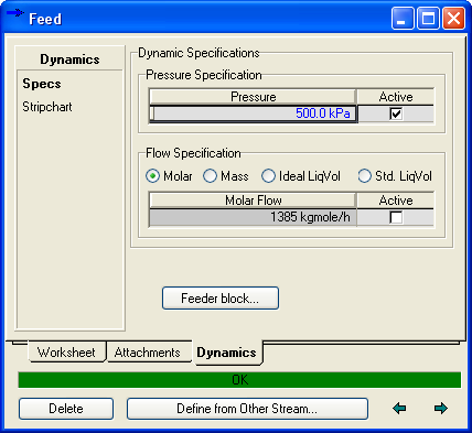
In dynamics mode, pressures are usually only specified on boundary streams (feed and product streams, which have no unit operations upstream or downstream) with the pressures and flow rates inside the model then a function of the equipment and contents of that equipment over time.
In steady state you make a specification by possibly deleting another specification, and then specifying a value for an EMPTY cell or by changing the value for an existing specification. In dynamic mode this approach just helps you to provide some values. You explicitly choose what is a specifications by clicking on the appropriate checks boxes on the dynamics tab of a unit operations view:


Flow rates can be specified as well, but that is only occasionally done for a feed stream (such as a vessel or column feed), or for very simplistic column models where the recycle flow rate is specified.
Why is this not recommended? Directly specifying or controlling the flow rate of a stream is not possible in practice. While it can certainly be done inside the model, doing so can lead to unrealistic behavior. For example, the flow rate may go against the pressure gradient. Or if the flow rate is typically liquid but ends up being vapour at some point because a vessel drains, then a mass flow rate specification can result in a sudden large change in pressure because the stream density changes. For these reasons, it is best to control flow rates by manipulating a valve or some other piece of equipment, as would be done in real life.
Material generally flows in a certain direction at a certain rate because there is a pressure gradient (driving force) and some sort of resistance (e.g. a pipe). It never flows against a pressure gradient and there is usually some sort of resistance.
Many pieces of equipment allow a pressure drop to be specified, but this is rarely done. Instead of setting a valve to use a fix pressure drop, it often makes more sense to size it and have it operate it is would in real life. Pressure drop specifications are common in steady state model, but generally avoided in dynamics mode.
A dynamics model tends to adhere closely to these concepts. It is possible to set up a model where these fundamentals are ignored for simplicity sake (e.g. flow with no pressure gradient, or excluding valves and such from a model, commonly done in steady state), but such details can be important if realistic behavior and responses are desired.
How much detail you have in your model depends on what you are trying to achieve with your model. The following diagrams illustrate some specifications and equipment that can be used around the simple vessel discussed earlier.

In configuration A, note that the pressure specification can be placed on any of the three streams. The outlet flow specification can also be moved to the other outlet stream. As discussed earlier, this configuration is of limited use.

Configuration B is more meaningful. The level is being controlled via a valve. This configuration, without the controller, could be used for example to determine how long the vessel would take to drain under gravity.

Configuration C shows a system where a vapour-liquid feed flow rate is being controlled, and level and pressure of the downstream vessel are being controlled. Optionally a duty stream can also be added and used to control the temperature.
Backwards Calculations and Flow Reversal
Steady state provides some support for backwards calculations or solving a unit operation from its products. In dynamics, if a stream has a positive flow rate, then its contents are always determined by whatever is inside the unit operation out of which it flows.
Dynamic mode also supports full flow reversal, and composition and other properties will propagate fully, as they would in real life.
Start Values
While in dynamics mode with the integrator not running, Petro-SIM will not exhibit the same behavior as in steady state. When a stream is connected to a unit operation, it will typically be initialized from other streams attached to said unit operation, even if the unit operation is not yet fully configured. This will provide it with a starting point for integration.
Inconsistencies
If too many specifications are given in steady state, the solver tends to stop and an error message about inconsistent specifications usually pops up.
This does not happen in dynamics mode. Each unit operations contributes some equations to the simultaneous solution and that system of equations may be over or under specified, but this can usually be readily understood and remedied and several helpful tools are available. Additionally, the contents of streams are usually determine what the unit operation out of which they flow, regardless of other considerations.
Dynamics mode will update the value of a specified (or even calculated) variable and not trigger an inconsistency. For example, a spreadsheet can export to a stream pressure which is marked as a specification and has a specified value, and will update that value. There is no need to delete the stream pressure value before exporting. And when a Set operation is set up, its target variable value should not be deleted before the connection is made, since the Set operation will adjust and update the target variable value (which should typically be a specification).
In dynamics mode everything should have a value when the integrator is started, and existing values are then updated as appropriate.
Table of Contents
Petro-SIM ships with several sample cases. Click on the "Open Sample Case"  button on the button bar (or click File, Open, Sample Case) to load a sample case. This section contains a brief description and comments on these cases.
Dynamics Debutanizer

This case demonstrates modeling a distillation column with more detail around the condenser. Column pressure control is handled by bypassing some of the overhead vapor around the condenser. PIC-101 controls the overhead accumulator pressure using the bypass. The top tray pressure is controlled by PIC-100, which essentially maintains a constant pressure drop between the top tray and the overhead accumulator. If the system overpressures, PIC-102 will vent to flare.
The reflux rate is on flow control, with the overhead accumulator level being controlled by the product rate. There is temperature control at the bottom of the column, and level control for the sump.
Additional item(s) which could be modeled are relief valves - probably one at the top of the column, and one for the overhead accumulator. The bottom product could be put on analyzer control, cascaded to the temperature control.
Dynamics Ethanol Dehydrator
This simulation demonstrates a simplified dynamic simulation of a three-phase chemical column. In this example, all of the organic phase from the decanter is refluxed to the column. In addition, a small amount of the aqueous phase is refluxed to maintain temperature control at the top of the column (TIC-100). The amount of aqueous reflux is insufficient to produce a second liquid phase on the trays.
Dynamic Glycol Reactor
This model simulates a glycol reactor with level and temperature control.
Dynamics Crude Distillation

This crude column distillation model was adapted from a standard steady state sample case Standard CDU.ksc. The flowsheet has been kept as close to the steady state flowsheet as possible. Because of this, for instance, there are no column sumps, except for the reboiled sidestripper. The case also does not utilize static head contributions and the control scheme is incomplete.
A model which is expected to go through startup and shutdown calculations will likely contain additional controls and details not included in this model.
Table of Contents
Steady State versus Dynamics
The same modeling environment is used for steady state and dynamics. It is possible to adapt an existing steady state case and use it in dynamics mode. In many cases the lined out dynamics model will provide the same results as the steady state model.
However, as demonstrated in the Key Concepts section, there are several fundamental differences between steady state and dynamics models. Due to static head considerations and specifications that require simultaneous solution, switching a complex dynamic model, especially one that has been built or extended in dynamics mode, to steady state, will require modification to solve successfully.
Once a case is in dynamics mode, the general practice is to keep it in dynamics mode and not switch back to steady state again. After all, the dynamics solver can also provide a lined out steady state solution in dynamics mode.
If a steady state model is to be transitioned to dynamics mode, the following should be kept in mind:
- Make sure the model is fully solved in steady state. This will provide a solution from which the dynamics mode integrator can continue.
- Consider where extra equipment such as valves or pumps may be required.
- Consider the size of equipment such as vessels and tray sections. In steady state the size of a vessel is often not relevant, but it can be a key factor in dynamics.
- Consider setting elevations where static head contributions will be relevant.
- Consider the pressures in the model. Steady state models often disregard pressure drops or have the same pressure throughout the model. Rectify this.
- Depending on the model complexity and specifications you choose, you may also need a control strategy. A simple model will likely not need a control strategy, but will possibly also be less flexible because of that.
You can use the dynamics assistant tool (described under Tools) to examine your model and get an idea of what changes may be required.
Building
The best way to develop a large model is by doing so in incremental steps. Start with a smaller model that runs fine. Then add onto it, and run the integrator to make sure it behaves as expected. Then add another section and so on.
Do note that you do not need to use recycle unit operations in dynamics mode. In dynamics mode, when a specification is changed or deleted, the case will also not forget (erase) values. When the integrator is started the model will always continue from the previous values, using them as a starting point. There are a few exceptions, such as the stream which will erase some values if you delete a specification, such that another specification can be made.
A Simple Model Step by Step
As an example and to illustrate some concepts, here is a simple model, to be constructed next:

Follow these steps:
- Create a new case. Since this is a level control exercise, we shall need vapour and liquid. Click File, New, Case. Create a component list and add N2 and n-Octane to it. Exit to the build environment. Note that clicking on the new case icon
 on the button bar will open a standard starting case which includes many component. You can make use of that case, intended for steady state refinery modeling, if you wish, though in general, for speed, you want to eliminate components that are not needed.
- Click on the dynamics mode button
 to switch to dynamics mode. This will ensure that dynamics mode specific pages are visible in the unit operation views.
- Now create a stream in the PFD. Hit F4 to open the palette if need be, and using the left or right mouse button drag a blue stream to the palette. Or double click on the stream icon in the palette to create a stream.
- Double click on the stream in the PFD to open it. Specify a pressure of 101.325 kPa, a temperature of 25 C, a flow rate of 1 kgmol/hr and set the composition to 0.5 mole N2 and 0.5 mole n-Octane. The stream will flash and solve.
- Create a vessel (Separator) and connect the feed to it. Also attach vapour and liquid streams to the vessel. Note that, since the integrator is not running, the vessel does not solve. But when you connect new streams to it, it initializes those steams from the feed stream. This will provide a starting point for the integrator.
- Go to the vessel rating page and specify a volume of 1 m3.
- Attach a valve to the liquid outlet stream. Note how the valve shows red, indicating that it needs to be sized.
- Open the Valve view on the Dynamics, Specs page, enter a Cv value of 0.5.
- Now the static head contribution from the liquid level should provide a driving force for the liquid, but open the Valve outlet stream. On the Dynamics, Specs page, check Active for pressure, and change the value to 91 kPa. Go to the vessel top outlet and also set the pressure specification for on. For the vessel feed stream, disable the pressure specification. There can only be one pressure specification among all streams directly connected to the vessel.
- Now at this point the model can be run, but the vessel will likely drain empty or overflow (either of which is fine).
- So add a controller from the palette. Open its view. On the Connections tab, set its output to be the liquid valve. Set the controller's process variable to be the vessel's liquid percent level. On the Parameters tag, set the PV minimum and maximum values to 0 and 100. Set the tuning values Kc to 1.2 and Ti to 0.4 (just as initial rough guesses, feel free to try and improve upon these later on). Finally set the controller mode to auto. Set the controller action to Direct.
- Now it would be nice to have a strip chart, so that we can monitor the controller. Open the vessel view and on the Dynamics, Strip Chart page, select "Small Dynamic" from the drop down. Then delete all the variables that show up, except Liquid Percent Level. Click Create Stripchart. On the controller, Parameters tab, use the right mouse and drag the OP value and drop it on the strip chart. You can access the stripchart settings in the Databook (press Control-D).
- Now run the integrator by click Go
 on the button bar, or press Control-I to open the Integrator view and click on the Start or Continue button.

Note how the vessel level is zero initially (since it is set by default to do a dry startup). The controller initially closes the valve which lets the vessel level rise. Once it start getting around 50%, the controller will start to open the valve.
- Later on, similarly, stop the integrator again. You can not add operations or delete them or change connections while the integrator is running.
- Now, lets add a pipe unit operation. Create one from the PFD and connect it up as shown. Attach an energy stream to the pipe and specify a value of 0 for it. On the Valve outlet stream, on the Dynamics, Specs page, uncheck Active for the pressure. On the pipe outlet stream, check the Pressure specification as Active, and set it value to 81 kPa. Now open the Pipe view. On the Rating, Sizing page, add one segment. Set it length to 10 m and the outside diameter to 8 mm and the inside diameter to 7 mm.
- Now start the integrator.
Note that the simulation will run more slowly because of the pipe unit operation. In many cases pipe sections can be ignored, or can be modeled more efficiently (but using a much simpler model) via the pipe option in the valve unit operation. It can be accessed on the Dynamics, Pipe page of the valve view.
The dynamics assist may come up during this exercise, depending on your preferences. It is discussed in the |Tools section. For now just dismiss its dialog boxes or choose to proceed in any event.
Various tools are available to help build models:
There are also tools to perform certain tasks on a model:

Table of Contents
Introduction
The integrator view can be access by pressing Control-I. It is also available under the Simulation menu. It allows the integrator to be started or stopped, and provides access to various options.
General Tab
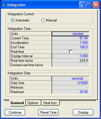
The integrator can be run in Automatic or Manual mode. In Automatic mode it will run indefinitely or until to End Time time is reached. In Manual mode it will execute a given number of time steps. Manual mode can be used for troubleshooting to slowly step through an event. It can also be used to temporarily pause the integrator without stopping it.
While the integrator is not running, the Current Time can be changed or set back to zero. This is equivalent to pressing "Reset Time". Note that this option will merely reset the time, it will not cause the model to reset or reinitialize. It will continue as before. Resetting the time this way is handy if it has run up to a very large number, or if the Event Scheduler has been configured to trigger actions at a given time.
Normally the integrator will run as fast as it can. If the "Real Time" option is checked, it will slow down to run at real time. It can also be made to run a multiple of real time. This is handy if time needs to be synchronized with another application or monitoring station or front end.
The default integration step size is 0.5 seconds. In some cases changing this value, especially to a very large value, can result in model instability under some circumstances. It is highly recommended that the default value be used in all situations. If a model exhibits stability problems, it is better to understand the reasons and change the model appropriately (usually this can be readily done), rather than change the step size. Also keep in mind that the model itself may be stable, but exhibit changes and transients that suggest instability, but are really proper behavior given the model and control configurations. The effective integrator step size is constrained to be within the minimum and maximum limits specified.
The integrator uses a fixed step size. Combined with the hybrid solver approach, this results in the best combination of stability and speed.
Topology changes, i.e. changing connections or adding or removing unit operations, can only be done while he integrator is not running. Making a topology change will cause the integrator to stop. The integrator can also be started by clicking on the Go button.
Options Tab

These options are all advanced options, and should generally not be changed unless there is really good reason.
The only exception is the Static Head contribution option, which should generally be checked. It used to be disabled by default in some older cases. Note that changing this option in an existing case may result in pressure and flows changing throughout the model.
The Execution Rates determines how frequently certain calculations are performed. If "Use these default periods for all operations: is unchecked, you can change the settings for individual unit operations. To access these, go to the Workbook and add a page for Dynamics Equipment Ops.
Heat Loss Tab

This temperature is used in the heat loss calculations in vessels, tray sections, and other equipment.
Table of Contents
Introduction
The dynamics assistant can be activated by pressing its button on the button bar  or by clicking Tools, Dynamics Assistant.
The main purpose of the dynamics assistant is to ensure that a sensible set of pressure flow specifications is selected and that new users are educated. After analyzing the case, it will recommend a list of changes along with an explanation of each group of changes. In addition, the assistant will also identify potential trouble spots in the case.
The recommendations of the assistant are intended to ensure that the case does not have too many or too few or incompatible stream pressure and flow or unit operation specifications. It looks at specifications which contribute equations to the simultaneous solution only, to ensure that the solver is able to solve and integrate.
For example, if you have a case with a valve and a feed and product streams, and you place a pressure specification on both streams and change the valve to use a pressure drop specification, the resulting equation set is not solvable. The dynamics assist would recommend changing the valve to use a pressure flow equation rather than a pressure drop equation.
The recommendations of the assistant may not always apply or be appropriate for every case. It serves as a learning tool for new users. When you no longer need the assistant, you can disable it via the preferences. The assistant is usually disabled by advanced users since it then no longer serves any purpose.
View
The General tab of the assist view looks as follows:

It shows a list of issues that have been identified in the current case. You can review what the assistant reports without making any changes. To have the assist make its recommended changes, click the "Make Changes" button. You can also select what groups of changes you want made. Click on the green check mark to enable or disable a group of changes.
You can double click on an item on the first page to see more details about it:

On the more detailed view you see exactly what the assistant wants to change. You can double click on a name to open the view for the affected unit operation. You can also uncheck the OK option for individual items if you do not want the assistant to change those items. You can also click on "Tell my why..." to get an explanation of why the assistant recommends the change.
Approach
The approach the dynamic assistant takes is loosely based on this philosophy:
Table of Contents
Introduction
The equation analyzer is an advanced user tool. It allows the user to view the set of simultaneous equations. Why? Situations where there are too many or too few specifications can be analyzed (though that is rarely needed). If the solution is singular, or if the equation solver fails, then this tool provides information about which equations (and hence unit operations) may be causing the problems.
This is not a tool that you should expect to use much. Petro-SIM strives to make dynamics robust and easy to use, without users having to be concerned about solver failures or such implementation artifacts. If you do get pressure flow convergence failures in Petro-SIM, please send the case in to KBC.
You can access the equation viewer by clicking Simulation, Equation Summary View.
Main View

Full and Partitioned Analysis are two options to analyze equations and find redundant specifications or missing specifications. If one option does not provide something useful, try the other. These two approaches work by analyzing the simultaneous equation matrix and possibly changing (partitioning) equations to facilitate better identification of problem areas.
The dynamics assistant can be used as an alternative to study over or under specified problems. It relies on a general approach rather than analyzing the equations. The PFD also has an option to show which streams have flow and pressure specifications.
The general equations tab contains a list of all the equations that the integrator solves. Double click on an equation to see more details for it.
If applicable, unconverged equations are shown on the Unconverged tab. This allows you to see where in the flowsheet the problem may be. Unconverged equations usually result from unusual situations, such as a spreadsheet possibly specifying a pressure of 1e11 kPa.
Table of Contents
Introduction
The event scheduler allows tasks be scheduled to execute when certain conditions are met. This can be used to perform simple tasks, or perform complex logic such as shut down operations. Please also see the Cause and Effect Matrix.
The event scheduler can be accessed by pressing Control-R or by clicking Simulation, Event Scheduler.

The event scheduler works by having a list of schedules. Each schedule can have a series of sequences. Each sequence has a list of events. Each event has a condition with a list of actions.
Schedules

Sequences have to be started (press Start) before they will be active. They will then remain active until all sequences have been completed, or the Schedule is Stopped or Held.
Sequences

Every sequence has a list of events.
Events

Each event has a condition which must be met before the associated actions are executed. Conditions include a specific simulation time, an elapsed amount of time, a value to stabilize, or a logical expression.
If a logical expression is used, variables from other unit operations can be added. These variables, using the Tag field, can be used to form the logical operation. The logical expression uses the same syntax as the spreadsheet.

Once the condition has been met, the actions are executed. Actions include specifying a variable (e.g. changing a pressure, closing a valve, shutting something off), starting or stopping another sequence, playing a sound, playing a script, or making controller changes.

The event can also be configured to jump to another event. This branching allows more complex logic to be configured without having to duplicate events.
Access the Control Manager by clicking Tools, Control Manager.

It provides quick access to all controllers in the case. It is easy to see which controllers have not reached their setpoint and to investigate, or to change the setpoint for several controllers at once.
The user variables tab is common to many views and allows you to define custom variables with values. It could be used to store previous setpoint or other values, but its uses is optional.
Table of Contents
Introduction
This functionality can be accessed by clicking Flowsheet, Dynamic Initialization. It allows you to define groups of objects and then performs certain actions on those objects such as reinitializing them all with Nitrogen.
Regions
You can create a number of regions, with each one typically referring to a collection of related objects. There are two ways to define a region:
- Click Flowsheet, Dynamic Initialization. Enter the name of a new region. A view will open for that region. Go to the Object page and click "Edit Object List". This will allow you to easily add objects to the region.
- Select a groups of objects in a PFD, right mouse click, and choose Send to Dynamic Initialization. This allows you to add objects to an existing region or send them to a new region.

Settings
On the Fluid Packages tab, an initialization stream can be selected. One can be selected for each fluid package, and the stream conditions and composition can be viewed. With a stream selected, clicking Initialize will fill all objects in the region with the stream. This is an easy way to clear out the contents of a plant by filling it with nitrogen before doing a dry startup for example.

On the Configuration page, other actions can be selected.

These actions include:
- Resetting valves to their fail state.
- Turn pumps off.
- Turn of air cooler air flows.
- Reset compressors (reinitialize them).
- Initialize controllers to manual with an OP of 0.
- Reset digital operation that have no PV to an output state of False.
- Run a user variable macro. The a user variable with the name given is found in any of the objects, its associated code will be executed. This provides a mechanism to perform custom steps or changes.
Table of Contents
Introduction
Many unit operations and streams have a user variable page where user variables can be added. Such variables can be used to store values, but can also be used to execute code scripts.

Variables in Dynamics
User variables can be created and edited exactly the same way as in steady state. However, do note the following issues which are specific to dynamics:
- User variables in unit operations and logical operation may contain code which can be set to execute. Stream user variable can be used to store values, but can not execute code.
- To have a user variable execute in dynamics mode, in the Script dialog box scroll through the list of check boxes and for check one of the following:
- Enabling or disabling a user variable is detected when the integrator is started.
DynExecute is available for logical operations, and the other two for material transfer operations (such as a valve or a vessel). DynCompositionPreStep will result in the variable being executed less often than selecting DynPressureFlowPreStep.

Do note that user variables with scripts that execute, while optimized, may slow a simulation, especially if the script performs complex actions such as creating and flashing fluids. Script are however handy for calculating something non trivial or triggering some action or communicating with external software. If a script merely performs a simple calculation, then using the spreadsheet instead will result in better performance.
The language used by default is VBScript and there are many internet tutorial sites which explain the syntax. Scripts can also be made to use any installed active script language by changing the very first line in the script to something like: language="JavaScript". Do note that the script language of choice needs to be installed on any computer where the model will run.
User variables by default have access to the properties of the object to which they belong. For example, a user variable in a controller can have code like this:
Pressing  will show a list of OLE properties for the controller.
Additional general information about user variables is available in the Petro-SIM F1 online help.
Table of Contents
Introduction
The Data Book (accessible by pressing Control-D, clicking Tools, Data Book, or clicking on  ) allows you to add variables and then do something with those variables, such as add them to a strip chart or record all their values.
In addition to browsing for variables from the data book view, variables can also be easily added by selecting them in a view, right clicking and choosing to send the variable to the data book. The latter is often easier than browsing.

Process Data Tables

Process data tables is one mechanism by which large amounts of data can be efficiently retrieved from or sent to Petro-SIM via OLE. The simulation case OLE interface provides a list of DataTables.
Strip Charts

A number of strip charts can be defined. For each the variables to be plotted can be selected. Various options such as how many points to store, how often to record a point, etc. can be set. The strip chart values can also be viewed or exported to a file.
The variables are plotted as a function of time and the strip chart will update as the integrator runs. Strip charts are very efficient and have minimal impact on the speed of the simulation.
A visible strip chart view itself offers many options accessible via the the mouse. For example, a variable can be easily added by right mouse dragging it from a view and dropping it onto the strip chart (the graph itself, not the databook). A right click menu is also available which allows various details to the set. By holding the left mouse button down on a strip chart, you can move or drag the strip chart to change what is visible. A trend can also be dragged up or down to make more of it visible.
Data Recorder

The data recorder allows you to select variables of interest, and then periodically, at will, record their current values. The values can then be viewed as a plot or as a table.
Case Studies
The case study functionality operates in steady state mode and is not used in dynamics.
Table of Contents
This section contains more detailed documentation for specific unit operations.
Material Transfer Operations
Palettes (F4)
- Mixer
- Tee
- Pump
- Compressor and Expander
- Vessel Reactors
- Plug Flow Reactor
- Flowsheets and Columns
- Tray Section
- Heat Exchanger
- Multistream Exchanger
- Heater Cooler
- Air Cooler
- Fired Heater
- Relief Valve
- Component Splitter
- Recycle
Logical Operations
Streams in Dynamics Mode
Streams behave similarly in dynamics mode as they do in steady state mode. But when a new stream is created or connected to the flowsheet in dynamics mode, it is typically initialized with starting values. Streams must have initial values when the integrator is started. The dynamics assistant can be used to easily fix streams which somehow do not have proper initial values.
Stream values are updated only when the user interacts with directly with the stream, or while the integrator is running. Changing a unit operation will typically not change any stream contents until the integrator is started.
The flow rate and pressure of a stream are either specifications (set via check boxes on the Specs tab of the stream), or are determined by solving a subset of simultaneous equations from the model, as explained earlier in the basics.
The stream conditions (temperature, enthalpy, phases etc.) are determined by the stream itself, or by the equipment to which it is attached. If a stream is a product attachment (outlet) and has a positive flow (greater or equal to zero), or it is a feed attachment and has a negative flow (less than zero), then its contents are determined by whatever unit operation feeds into it. The stream phase fractions will also depend on that unit operation. The values may depend on the liquid levels inside that unit operation and the stream nozzle elevation and diameters, as explained earlier in the basics. The stream phases may or may not be in equilibrium.
If a stream has a positive flow rate and there is no unit operation upstream of it, then its conditions and composition are as determined by the stream specifications (on the conditions and composition pages of the stream view). These can be set while the integrator is running or while it is stopped. If a product stream attachment, which has no unit operation downstream connected, has a negative flow rate, then its conditions and composition are also set by specifications inside the stream. So a product stream with a negative flow rate behaves exactly like a feed stream. And a feed stream with a negative flow rate becomes a product.
Note that during the simulation a stream's flow rate may change direction. If a feed stream has a positive flow rate, reverses flow, and then changes back to having a positive flow, its composition and conditions are determined by the stream's feeder block. A feeder or product block is present in any stream that is not connected at both ends. Think of the feeder block as an infinite vessel. Its contents does not change if material flows into it, and it always provides the same predetermined contents to streams that flow out of it.

If the user changes conditions in a stream (e.g. specify a different temperature or composition) then the feeder block will update its values with those from the stream. The user can also explicitly set values inside the feeder block and export those to the stream.
Note that, while not possible in steady state, it is possible to export composition values from a spreadsheet to a feeder block or stream in dynamics mode. The feeder block will automatically detect full or partial composition specifications and trigger an update in the stream, depending on its flow rate. Condition specification sent to the feeder block. The feeder block will then pass them to the stream, as and when appropriate.
Since stream flow rates are determined from a network of equations, composition specifications should be on a mole or mass fraction basis for example, rather than on a flow rate basis.
The conditions page of the stream has an "Initialize Stream Conditions" button. When pressed, it allows the use to specify any stream conditions (temperature, enthalpy etc.) regardless. The stream will flash (recalculate) if a value is specified. This can be used to change the contents of a steam anywhere in the simulation, if need be. Of course once the integrator starts, the stream will likely be updated by attached unit operations. But there are some rare situations where it is desirable to change a stream or perform a quick experiment.
Do note that terminal (i.e. having no upstream or downstream operation) streams typically have pressure specifications. Such stream are also typically connected to something which has a pressure flow relationship such as a valve. Terminal streams that instead are directly connected to a vessel can also have a pressure specification (e.g. a vessel vapour stream which opens the vessel to the atmosphere), but only one terminal stream directly connected to a vessel can have a pressure specification. Internal (non terminal) streams generally do not have pressure or flow specification, as their flow and pressure are determined by the network equations. If a terminal feed stream is directly connected to a vessel, it will typically have a flow rate specification.
Do note that terminal feed streams without a pressure specification may continually flash (recalculate) as the pressure changes. This can be costly in some cases. This situation can be avoided by inserting a valve and specifying its upstream pressure instead of the flow rate and using the valve to regulate the flow rate.
Introduction
In steady state the valve is only occasionally used, typically with a specified pressure drop. But in dynamics mode the valve is a key unit operation. As in real life, it is used to regulate flow or pressure. It is a fundamental building block in that it establishes a relationship between flow rate and pressure gradient, which results in a realistic model. In dynamics mode the valve is nearly always set to use a flow equation rather than a fixed pressure drop.
Sizing
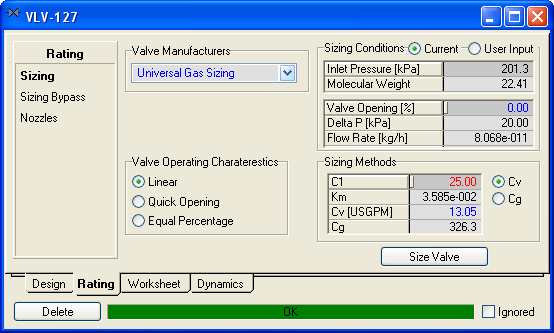
For valve manufacturer the choices are:
- Universal Gas Sizing - The flow rate is linked to the frictional pressure gradient according to the Fisher Controls Universal Gas Sizing Equation. This includes vapour choking, where the flow rate may at some point stop increasing if the pressure gradient continues to increase. Liquid choking is not currently modeled.
- Simple Resistance Equation - The flow rate is proportional to the square root of the frictional pressure gradient. There is no choking.
The valve operating characteristics allows the valve control type to be selected:
- Linear: Valve travel is directly proportional to the valve stoke.
- Quick opening: Large increase in flow with a small change in valve stroke.
- Equal Percentage: Equal increments of valve travel produce an equal percentage in flow change.
The default is linear, though equal percentage is perhaps the most commonly used valve control.
The valve opening can be changed on this page so that it can be used to size the valve. In general, do not try to directly control or manipulate the valve opening with a spreadsheet or controller, but rather manipulate the valve actuator desired position (which will drive the valve towards to desired position, factoring various other considerations as well).
The valve can be sized from the current conditions (e.g. if it was just added and the outlet pressure was updated), or from a set of user conditions.
You can also choose what combination of Cv (valve liquid size coefficient), Cg (valve gas size coefficient), Km (pressure recovery coefficient) and C1 (C1 = Cg/Cv) to specify but all four values must be determined. By default C1 has a value of 25 (ranges from 16 to 37 generally) and Km = 0.001434 * C1.
The valves comes with sufficient default options and values, and at minimum a new valve just needs the Cv to be specified.
Sizing Bypass

If Model Valve Station is checked, then a bypass valve and block actuators are also modeled. The bypass valve acts exactly like another valve in parallel with the main one. It is common enough that it is directly supported by the valve without to actually use another valve instance.
Nozzles

The nozzles page allows the valve elevation and inlet and outlet nozzle elevations to be set. These are used in static head calculations. The diameters are used if the valve is also modeling a section of pipe.
For operations like valves, the feed and product nozzle elevations are generally left to default to the same elevation as the valve. However, they may be changed to introduce artificial elevation differences in the absence of detailed additional equipment.
Specifications

The valve contributes equation to the simultaneous pressure flow network. It can add an equation which fixes the pressure drop across the valve, as well as a flow equation which links flow to frictional pressure drop. In most situation, (only) the flow equation option will be used, since it is most realistic.
This view also shows the valve size and relevant values and can be used to size the valve based on current values.
Checking Check Valve will prevent reverse flow through the valve.
Pipe

The valve can also be used to model as section of pipe. This pipe model performs a relatively simple and fast calculation, but is sufficient in most cases to model the pressure loss associated with a section of pipe.
It calculates a friction factor using the information provided and uses that to add a contribution to the valve flow equation (which must be used to be able to model a section of pipe). Assuming turbulence results in slightly faster calculations because the friction factor is fixed. Turbulent pipe flow is common.
Note that this pipe model may not provide accurate results for multiple phase situations and does not model choking or any complex transient phenomena such as shockwaves.
The Disable Valve can be used to model a section of pipe only, with no valve. This is handy for solving pipe network systems or studying a vessel drain through a pipe under gravity for example.
The pipe option is generally used where the pipe can have a significant impact on flow or pressure. While it can be configured in every valve, there is typically minimal benefit in doing so.
Holdup

This view is common to dynamics unit operations and shows the contents of the volume inside the unit operation as well as other generic relevant information such as nozzles.
It is recommended that the valve volume be left at zero. Adding in a small valve volume results in more complex equations which is rarely worthwhile. It is often simpler to just increase the volume of a nearby vessel slightly if need be.
Actuator

A valve is made up of several components. Usually there is a control signal which is then used by an actuator to change the valve accordingly. This is important because actuators have a dynamic response, and also the actuator may stick or fail, and thus prevent the valve from reaching the desired position.
The actuator can be made to fail, and whether this results in the valve remaining open, shut, or staying at its last position, can be set on this page.
If the valve has worn trim, the it will not fully close.
Valves should be controlled by setting the actuator desired position, rather than the valve opening directly.
Actuator Station

If a valve station is modeled, then actuator settings for the bypass and main valves, as well as the block valves can be set here. The valve station can also model the action of two block valves in series with the main valve.
Stripchart

This view can be used to quickly create a stripchart. Select a group of variables from the drop down and then remove unwanted variables from the matrix before pressure the button to create the stripchart.
Table of Contents
Introduction
The pipe unit operation can be used to model pipe section where the pipe is very complex, makes use of heat transfer, has multiple phases, or experiences choking. Since the pipe calculation is more rigorous and costly, in most cases the pipe option inside the valve van be used. Also, avoid using a pipe unit operation for every possible section of pipe in the model, as doing so is usually redundant and time consuming and will slow down the simulation.
Note that the pipe does not model rigorous transient phenomena such a shock waves.
Pipe in Dynamics

The pipe is configured the same way as in steady state (press F1 in Petro-SIM for more help). Dynamics mode only require the elevation of the entire pipe section to be provided, since static head contributions between it and other equipment may be relevant.
To add a simple pipe in dynamics mode, connect it up in the flowsheet. Attach a duty stream and on the Rating, Heat Transfer page, specify the heat loss to zero. On the Rating, Section page, add one segment and sets it length and diameter. And that is it!
The pipe unit operation will provide the same results as it does in steady state.
Table of Contents
Introduction
This section covers the vessel unit operation, which refers to the separator, three phase separator, tank, condensers and reboilers.
Differences from Steady State
Vessels in dynamic mode behave differently than in steady state mode. Some of the differences include:
- Phases are not necessarily at the boiling or dew point in dynamics mode.
- Vessels can overflow and drain and all vessels can have up to three phases.
- Outlet phases are determined by flow direction, and nozzle elevation and diameter, as explained in the basics. So the vapour outlet can contain liquid if the vessel overflows.
- The phases are not necessarily at equilibrium. Dynamics mode supports efficiencies.
- The vessel size and geometry are very important in dynamics.
The vessels all behave basically the same way.
Parameters

For best realism, the vessel Delta P should be specified to be zero. Frictional or static head contributions for feed attachments should be properly modeled using elevations or valves or such. The feed pressure drop specification is always applied in dynamics mode.
The duty should preferably be controlled to maintain a desired temperature or composition somewhere, along with level control where applicable. Subcooling specifications are ignored in dynamics mode.
Sizing

In steady state the vessel size or geometry is often of little importance. But in dynamics mode this can impact the levels and how they and the pressure in the vessel changes.
Certain geometries support a boot. This is a smaller section at the bottom of the vessel, usually with a much smaller diameter and height than the rest of the vessel. It is generally used in three phase elevation so that a small amount of a second liquid phase such as water will have sufficient level so that it can be readily removed, rather than forming a think spread out layer at the bottom of the vessel.
The weir option may also be available for certain geometries. The weir inside the vessel divides it into two chambers. Chamber two is generally smaller and allows the lighter liquid phase to overflow so that it can be easily drained away instead of possibly forming a too think layer at the top of the vessel liquid.
Nozzles

Note that the contents of the vessel products are as determined by the levels inside the vessel and stream nozzle elevations and diameters, as explained in the basics. The elevations also impact static head contributions, when active.
Heat Loss

Depending on the type of vessel, the heat loss may be set to None, Direct Q, Simple or Detailed. Direct Q means that a fixed heat flow is specified. If the simple model is chose, the heat loss is typically calculated from
If the ambient temperature is not specified, the default ambient temperature value from the Integrator view Heat loss page is used (and also updated as it changes).
If the detailed option is chosen, then the equations are far more involved. This option allows Metal and Lagging properties (thickness, heat capacity and conductivity) to be specified. The thickness for either or both of these can also be set to zero if they are not present. The inside and outside convective heat transfer coefficients also need to be specified, with defaults provided.
In both cases the area is calculated from the vessel geometry.
The heat loss calculation and values are a separate issue from the vessel duty stream. The heat loss is applied to the entire vessel contents by default. If the vessel phases are not in equilibrium because of efficiencies then the duty effectively applies to the portion of the material that is flashed in equilibrium before being mixed back with the remainder of the material.
Level Taps

Multiple level taps can be added to the vessel. Each level tap can sense the elevation of one or two liquid phases inside the vessel, but it can only sense the elevation in a certain range (the PV High and PV Low). The tap may not be installed to extend the full height of the vessel, or may deliberately be set to only measure low levels at the bottom of the vessel. If the vessel is using a weir, then the level tap can also be installed in chamber 1 (before the weir) or in chamber 2 (after the weir).
The level tap input signal (coming from the level and PV high and PV low), gets converted to an output signal in the range of OP Low to OP Low. So the final value that is available to a controller say could be manipulated to be a percentage (in the range of say 0 to 100%) or to act like an actual level or elevation (in which the type can be set the Length for example).
Specs

When a vessel is newly created or has never been run yet, it will initialize its contents when the integrator is started. This can be done by combining the product streams and flashing. A dry startup can also be done. In this case the vapour inside the vessel is determined from the attached streams and is not set to be at its dewpoint as steady state would do. User specific initial values (a composition, temperature and pressure) can also be provided. Unless dry startup is selected, the initial amount of liquid is determined by the liquid volume percent. If two liquid phases are present, they are ratioed according to the relative amounts of the two phases.
Note that at any time, specifically while the integrator is not running, a value can be entered for Liq Volume Percent This will adjust the amounts of liquid and vapour in the vessel as desired. This is a quick convenient way to quickly change or reset the level in a vessel without having to wait for it to naturally change.
The fraction calculator (so called because it calculates the outlet phase fractions) can be changed from its default value of Use levels and nozzles to Emulsion Liquids. The emulsion calculator assumes that for two liquids, while still being immiscible, the phases are not separated. Both phases will exit the vessel for any nozzle that is underneath the top liquid levels.
Condensers also allow for a Reflux Flow / Total Liq Flow specification. This is only to be used in simple column models. Otherwise condenser sections should be modeled more rigorously as demonstrated in some of the Samples.
The Vessel Pressure can be made a specification in the network of equations that are solved simultaneously. This is determined by the state of the checkbox. The vessel pressure always appears blue, allowing the user to possibly change it or set it to an initial value before starting the integrator for example.
The Add/Configure Level Controller will install a level controller if one is not installed already. It will be connected to a valve in the main liquid outlet line if one is present, or to the stream itself. Rough initial tuning values will also be provided.
Holdup
This view is more for information purposes. It allows the details of exactly what is inside the vessel to be examined.
It also provides a way common to many unit operations of accessing elevation and various nozzle settings.
Nozzles and efficiencies are discussed in the basics.
StripChart

To easily add a strip chart, select a group of variables from the drop down, then edit the list of variables by deleting undesirable ones and click the button to create a strip chart.
Duty
The presence of the duty page depends on the presence of a duty stream.
If a gas heater is used, then the duty is scaled down as the level decreases and less heat is transferred to the vessel contents. If a vessel heater is used then the full duty is applied.
For a Direct Q duty source (i.e. use the energy stream value directly) the value may be provided, as well as a range for possibly scaling the duty based on level. This mode is commonly used in vessel to control the duty.
If the source is a utility, the duty is calculated and updated in the duty stream. The calculation is done using the flow and properties provided for the utility fluid. Pressing Initialize Duty Valve results in the duty valve using the current vessel temperature and energy stream duty to calculate temperature and UA values for the duty fluid so as to result in similar duties being calculated as when only the energy stream was used directly. This makes it easy to switch to using a duty fluid, whose effect can be controlled by manipulating its flow rate.
Condenser specifications such as degrees of subcooling are not supported in dynamics mode because they are pure design specifications. Instead the temperature inside the vessel needs to be controlled.
Table of Contents
Introduction
The mixer allows a number of stream to be combined together.
Mixer Dynamics

In dynamics mode, the mixer naturally supports reverse flow for any stream. The mixer will mix all steams to it that are effectively feeds (feed attachments with flow rate greater than or equal to zero, and the product if its flow rate goes negative), and the result will be propagated to all effective products.
One setting is provided on the Dynamics page. It is recommended that only the Equalize All option be used, as this is the most natural setting. The mixer is really just a small mixing point and at the point where the streams actually mix, they all really have the same pressure. Note that with this option streams may still show very different pressures, due the nozzle elevations and static head contributions and the fact that a stream is a sampling point located where it is a product attachment, as explained in the basics.
The Set Outlet to Lowest Inlet should not be used, since it only makes sense in steady state where some equipment is not modeled and hence some pressure changes are ignored by using this option. Dynamics will still try to comply with this option, but will continue to apply the effective option in place at the time when the integrator is started.
Table of Contents
Introduction
Similar to the mixer, the tee is a point where streams combine and diverge. It also allows splits to be specified for products.
Tee Dynamics
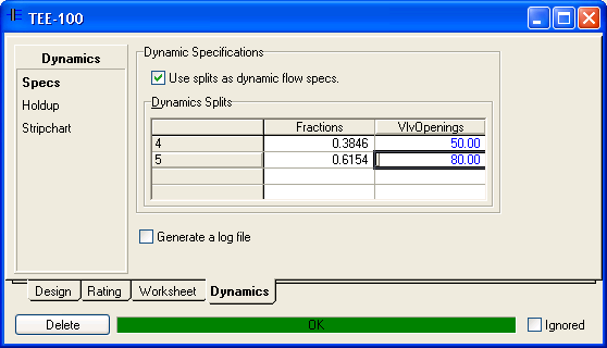
There is one option for the Tee which determines that equations are contributed to the simultaneous network. It is recommended that for larger more realistic cases and in general, that the Use splits as dynamic flow specs option be left unchecked. This is more realistic since the flow rates in the various streams will then be determined by the pressure and resistances through the model.
Alternatively, the product outlets can also be determined by specifying a valve outlet for every product. The ratio of the valve openings determine how much of the feed stream flow rate is linked to each product stream. These values can be controlled of course. This option should only be used for simple cases and setups, since it can result in unrealistic behavior such as flow against the pressure gradient.
Table of Contents
Introduction
The pump is frequently used to provide a driving force for moving liquid.
Curves
Steady state supports a pump curve as found on the Design, Curves page in the view. However, dynamics mode needs to support a more complex set of curves, as found on the Rating, Curves page. This is because modeling pump startup and shutdown requires a more complete set of curves.

If pump curves are used it is generally recommended that several curves (at least three or four) be adding, covering the range of speeds across which the pump may operate or go through. The code will extrapolate beyond the curves values, but this can be problematic in some situations. A healthy set of curves provides good results, since equations are contributed to the simultaneous solution for the curves.
NPSH

Net positive suction head curves can be provided so that the required pump NPSH can be determined. If the NPSH available is less than the NPSH required, then the pump cavitates. This is modeled by varying the density in the pump equations. NPSH curves do not contribute equations to the simultaneous solution.
The NPSH available is calculated from the flow velocity using the feed nozzle diameter. It is equal to the inlet pressure minus the vapour pressure in terms of height plus the velocity head.
Nozzles
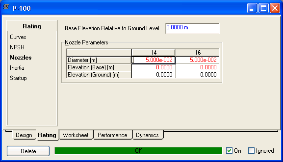
The feed nozzle diameter is used in NPSH calculations. The pump elevation is used to determine static head contributions. The pump nozzles are typically left to be at the same defaulted elevation as the pump, but can be adjusted to model additional elevation differences without adding extra equipment.
Inertia
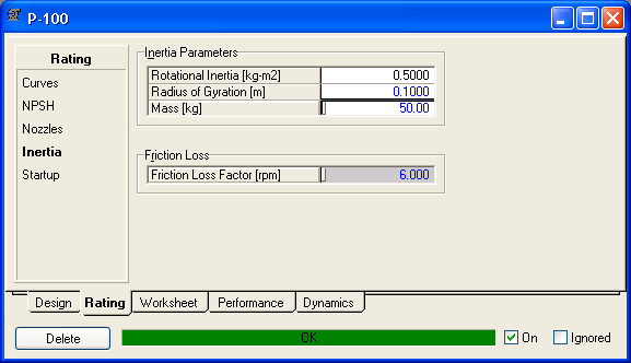
Modeling inertia can be helpful in realistic pump modeling and tends to make it easier to model pump startup and shutdown. Both inertia and friction result in a small duty loss in the pump.
Startup

The typical operating low is used by the pump to make some minor adjustments to densities and duties at very low flow rates (e.g. to avoid using a vapour density right at startup). An approximate or default value will suffice in most cases.
Performance

The pressure head is the total pump pressure change express as a height by using the feed density. The velocity head is the difference between the product and feed velocity heads. The two velocities are calculated using the nozzle diameters. Note that the total head also includes other contributtions such as the frictional pressure change.
Specs
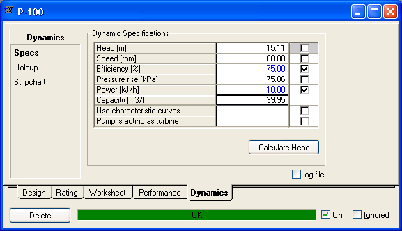
This determines what equations the pump contributes to the simultaneous equation network. By default the efficiency and power are specified. If Use characteristic curves is checked, then only one other specification (power is strongly recommended) is typically used since two equations are contributed for the curves.
Pump is acting as turbine can be used to model a turbine which generates power. The pump equations are still mostly the same, except the sign of the head is changed (since the pressure gradient is reversed), and the inverse of the efficiency is used.
Note that the pump can of course be switched on and off. If the pump has a speed specification, then this is done by ramping the speed up and down. If the power is specified, then the power is ramped up or down.
Table of Contents
Introduction
Compressors are similar to pumps in that they increase the pressure of a fluid.
Links

It is possible to model a series of compressors which are linked together on the same physical shaft. There can be one turbine in the link to provide the total power, or it can be specified via a negative value in the Total Power Loss. Modeling a linked train is usually very dependent on a good set of curves in each compressor. A linked set of units are typically all set to use curves (on the Specifications page) with no other specifications typically required in each.
Settings

If the compressor is in reciprocating mode, rather than centrifugal mode, the settings are available on this page. Positive displacement units do not make use of characteristic or flow restriction curves.
Curves

Since startup and shutdown can be modeled as well, a healthy set of curves covering the range of speeds is typically a wise idea if curves are used.
The curve page is only available for centrifugal units.
Flow Limits
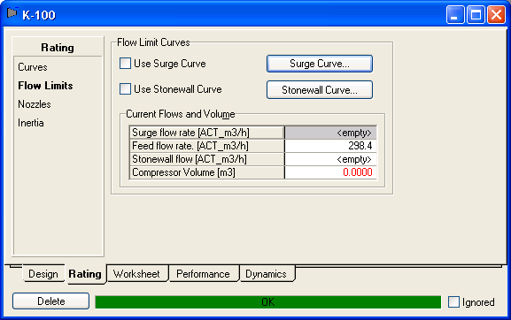
The flow limits page is available when modeling a centrifugal unit, but not when modeling a reciprocating unit. A simple stonewall or surge curve can be provided, usually two points in each suffices. These two curves do form part of the simultaneous solution. A warning will be displayed if the compressor approached the surging or stonewall operating limits. Stonewalling typically means that the flow rate will not increase any further.
Surging, where the compressor can not add enough energy to overcome system resistance, is modeling by adjusting the duty in the equations continually.
Some modelers choose to not use the surge and stonewall curves, but rather calculate their own values and display a warning in the user interface.
Nozzles
The compressor elevation is used to determine static head contributions.
Inertia

Modeling inertia can be helpful in realistic compressor modeling and tends to make it easier to model transients. Both inertia and friction result in a small duty loss.
Performance

The values displayed here typically match those of steady state, except that the duty loss due to inertia and friction is applied in dynamics mode only.
Specs
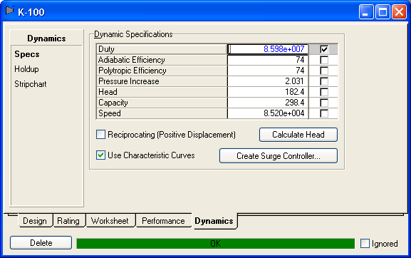
This determines what equations the compressor or expander contributes to the simultaneous equation network. By default the duty and polytropic efficiency are used as specifications. If curves are used as specification, then the compressor speed is typically used as a specification. However, if the compressor is linked to other compressors, then no speed specification is used and the speed is determined via the linked units.
The the Reciprocating option is checked, then positive displacement setting can be accessed on the Design, Settings view.
Table of Contents
Introduction
Vessel reactors refer to ordinary vessels where a reaction set can be attached, or to continuously stirred tank reactors such as the conversion reactor or CSTR reactor.
Vessel Reactor Dynamics
In dynamics mode these reactors are modeled very similarly to the way the vessel is modeled. They can have level control, level taps, etc. The main difference is that when the vessel flash continually as the integrator runs, reaction calculations are also optionally performed.
As an example, look at the Dynamics Glycol Reactor sample case.

Table of Contents
Introduction
The PFR is configured and set up the same way in dynamics mode as it is in steady state mode. However, the links between pressures and flow rates are set on the Dynamics, Specs page.
PFR Dynamics
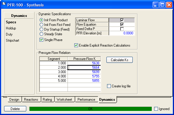
When a PFR is used for the first time in dynamics mode, the holdup volumes need to be initialized with some starting content. The options are:
- Init From Product which is the recommended default. The reactor is initially filled with product.
- Dry Startup (Feed) in which case the reactor is initially filled with feed material, but vapour only.
- Steady State can be used if the case was solved in steady state mode and now being used in dynamics mode.
As for pressure and flow specifications, the options are Flow Equation or Fixed Delta P. It is recommended that only flow equation be checked as this establishes a natural link between flow and pressure gradients. Fixing the pressure drop can be used in simple cases but in large models it can result in unrealistic behavior such as flow against a pressure gradient.
If Flow Equation is checked, then a k value needs to be specified for each segment. This k value is used in the equation which links the inlet flow for that segment to the frictional pressure gradient. Calculate K's can be used to calculate these k values from the current pressure gradient, density, and flow values.
Laminar Flow is checked by default and changes the pressure flow equation solved in the network to be simpler and more consistent with laminar (lower) flow conditions. In such cases the flow is proportional to the pressure gradient rather than the square root of it.
Single Phase can be checked if the contents is all vapour or all liquid. This will speed up reaction calculations, and should be checked when applicable.
Enable Explicit Reaction Calculations can be checked to use a faster method of calculating the reaction results. In some rare cases this may cause instability, but is generally preferred for speed.
Lag Rxn Temperature (visible in older views) is not used.
The duty option can be set similar to what is done for the vessel. The duty is typically divided and applied equally to the individual segments.
The number of segments can be changed while the integrator is not running. But if segments are added, K values typically need to be provided for those segments. While additional segments will result in a truer plug flow result, it will also slow down the model, as each segmented is flashed and reacted separately.
Table of Contents
Introduction
Both of these allow for a collection of objects to be organized as a combined group, conceptually.
Flowsheets in Dynamics
In steady state column flowsheets are special because they use a different solver to solve the entire flowsheet, and certain solvers only support certain configurations. In dynamics mode, the column flowsheet is no different than any other flowsheet and unit operations in it work and solve the same way as in other flowsheets. What is special about a column flowsheet though is that the tray section, condenser and reboiler operations can only be created inside a column flowsheet. Condensers and reboilers are covered in the vessels section.
In steady state it is common to interact with the main column flowsheet, but in dynamics, it is common to interact with the individual unit operations. So in dynamics mode, a tray section must be dealt with as a unit operation, rather than part of the column.
Table of Contents
Introduction
The tray section models a sequence of stages, each with a volume, liquid level, and flows between stages. Stages can individually flood or be run dry.
Sizing

The volume determines the amount of material on each stage, so it is important. Also, the weir length and height generally strongly influence the amount of liquid on each stage. The same values are used for all stages in the section.
Nozzles
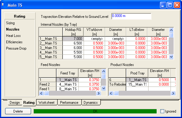
The elevation of the entire tray section can be set as can nozzle elevation and diameters for streams between stages and external streams. Nozzles for internal streams are usually left to the default elevation and diameter. For feed nozzles the elevations are sometimes changed so as to influence static head or the phases that will be withdrawn in the case of flow reversal.
Heat Loss

Tray sections generally lose heat to their surroundings and in some cases this can have a significant impact. Various degrees of detailed heat loss models are hence available.
Efficiency

Tray efficiencies generally set the stage recycle efficiencies (see | the basics) and can be used to model non equilibrium stages. While these can deliver similar results to steady state, the definition and values can differ. Tray sections are usually modeled as a series of ideal equilibrium stages.
Component efficiencies are not supported in dynamics.
Hydraulics

The page shows the tray static head contribution, the height of liquid over the weir, as well as the dry hole (vapour frictional) pressure drop.
Specifications
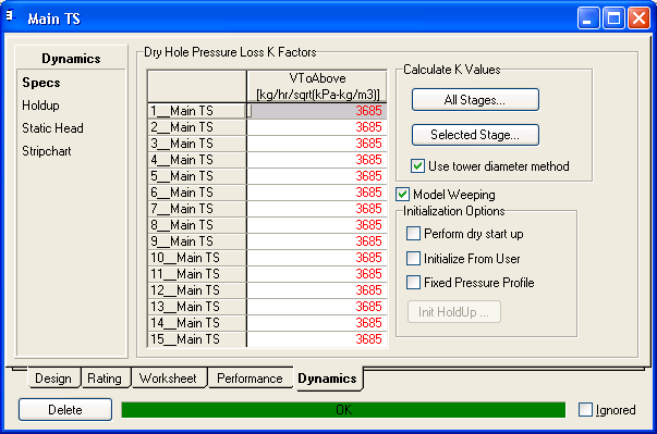
Each stage requires a K value, which links the vapour flow rate from one tray to the tray above it to the dry hole frictional pressure loss. The liquid flow rate is determined by whether the liquid height is higher than the weir height, or whether the tray is weeping.
Fixed Pressure Profile can be used to model very simple columns where changes in the pressure profile are not of interest. The stage pressures are all fixed.
Dry Startup and Initialize from User can be used to initially fill a tray section with vapour only or user chosen contents. Note that the dry startup option can be rechecked if the integrator is not running, allow the tray section contents to be readily emptied.
Static Head

For trayed sections, static head contributions are often essential for a realistic model and pressure profile, even if static head contributions might not be desired in the rest of the model. It can be turned on specifically for tray sections only, though most models have static head turned on in general.
Table of Contents
Introduction
The two stream heat exchanger model is commonly used in many models. If one side has a heating or cooling fluid, there is often a valve with a temperature controller on that line.

Model

A Basic and a Detailed model are available. In nearly all cases the basic model is used.
For the simple model, each side also has a volume which can provide some transient effects. The volume can also be set to zero, though very very small non-zero volumes are not recommended.
The overall UA value is always specified. It is strongly advised to also specify a reference (typical, normal) flow rate for both sides. If the flow drops below the reference value, then the UA value is scaled back down. This scaling can provide more realistic shut down and startup modeling and also avoid potential issues at lower flows. The UA will be scaled to no less than the given Minimum flow scale factor.
The detailed model is used only when a more rigorous model of the internal of the exchanger is desired:

The detailed model makes use of the rating information such as number of tubes, shell diameter etc. to create a network of volumes and heat transfer equations. The detailed model will run more slowly than the basic model. The Zones per Shell Pass determines in how many different sections the model is divided. It is fine to set this value to 1.
Specifications
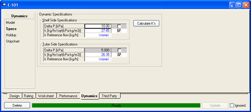
The overall pressure drop on each side can be made a specification by checking the checkbox for Delta P. However, as discussed in the basics, this is unrealistic, and as such it is better to always use a pressure flow relationship by checking the k option (only) for both sides and supplying a k value. Pressing Calculate Ks will calculate a k value from the current pressure drop and flows. For a newly created heat exchanger, sizing pressure drops can be provided by turning on the Delta P options temporarily to specify pressure drops to be used in the calculation.
If the detailed model is used, the Delta P Calculator can be used to calculate the pressure drop through the exchanger, but it is alslo possible to set it to "not specified" and then check the Use Pressure Flow K option. K values can be calculated by temporarily setting the Delta P Calculator to user specified, specifying a pressure drop, and clicking the Calculate Ks button. Details of the model can be viewed by pressing K Summary.
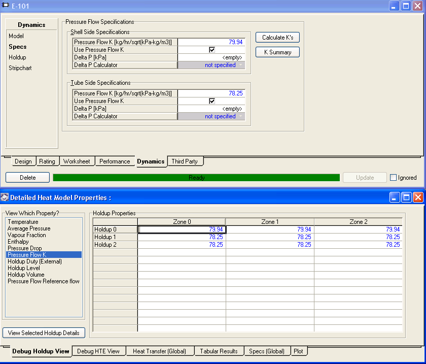
Table of Contents
Introduction
These heat exchangers consist of thin chambers separated by plates that route fluid through alternate hot and cold passages. Heat is transferred via the fins through the metal between the fluids.
Rating
Steady state solves the LNG by relying on a number of specifications such as UA, temperature or duty specifications. But dynamics mode provides a powerful robust fairly rigorous rating model. The model can be used for plate fin exchangers.
The model can be split into a number of zones (sections if you will), and a set of equations is written for each zone. Fluids can flow from a layer in one zone to a layer in another zone, and an external stream can enter into or exit from any zone.
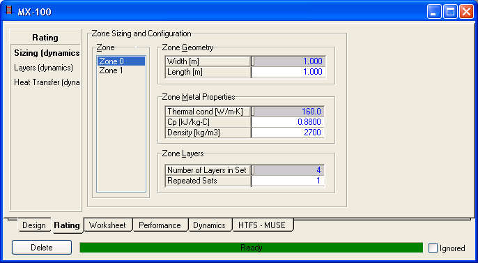
The sizing page allows the physical size of the zone (think of it a plate fin metal block) to be specified, as well as the properties of the metal.
For each zone a number of layers is set up, which provides a pattern for how stream are inside inside the unit. If the exchanges has only two streams, the set will likely have two layers since hot and cold will alternate. The set then repeats a large number of times. The total number of metal layers is equal to the number of sets multiplied by the number of layers in the set.
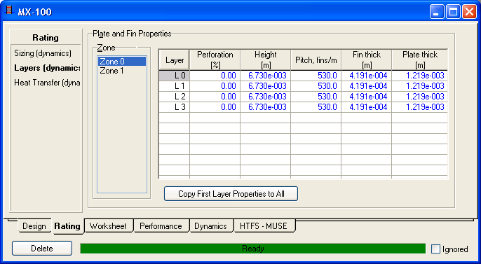
For each layer in the repeating set, the properties can be specified. These include perforation, height, fin pitch, fin thickness and plate thickness. These values impact the heat transfer area and geometry.

This page determines the heat transfer coefficients. These are typically specified and scaled based on the flow rate. They can also be calculated by setting the "U Calculator" to "Hysim Correlation". The area is automatically determined from other information provided.
Since the LNG can model startup and shutdowns and flow reversals and very low temperatures, reference flows should be provided.
Performance

The summary view can be used to get a quick overall look at what is happening inside the various layers and zones. It shows the temperatures of the fluids entering and leaving each layer.

The layers view shows even greater detail of a specific heat transfer point. Pressing Diagram shows detailed temperatures and duties at a specific point inside the model.
Model

The number of zones determines how many metal blocks, if you will, the exchanger has. Additional zones can be added for greater rigour. The zone is made of of a number of sets of layers that repeated. The number of layers in the set determine how the fluids are arranged inside the block. Typically a hot stream is located next to a cold stream.
For example, if the exchanger has two fluids, A and B, they will typically be arranged in alternate layers of hot, cold, hot, cold, hot, cold etc. One zone with two layers repeating can then set up. The same fluid may appear multiple times in the pattern , and possible have different temperatures in the different layer depending on its connections. By default each layer in the pattern is modeled in detail with a separate volume and set of heat transfer equations. The Combine Layers option can be used to combine these model entities for layers that contain the same fluid.
If the model is fully flexible in terms of zone and how they are connected. Some exchangers have very complex arrangements with some fluids passing through the entire exchanger and some only being present in certain zone. Each layer must have a feed and product connect. Each can be either an external stream connected to the exchanger, or another layer in any zone.
Click Auto Connect to automatically connect stream and layers to the zones, using a very simple approach. This is often handy to provide some initial values.
Specifications

A pressure drop calculator can be selected for each layer. As discussed, for most realistic results, this should be set to "not specified" and the Flow Equation option checked for all layers and all zones. K values can be calculated by specifying a value for Delta P and then pressing Calculate K's. If the Laminar option is checked it means that the flow rate is proportional to the frictional pressure gradient, rather than the square root of it.
Table of Contents
Introduction
The heater cooler is a simple means to heat up or cool down a single stream.
Specifications
Three modes are available:
- Supplied Duty - The value in the duty stream attached to the heater cooler is directly applied to the fluid.
- Product Temp Spec - The fluid passing through the unit is heated or cooled to exactly the given temperature.
- Duty Fluid - Models a very simple heating or cooling fluid.
Heater coolers are handy in small or simple cases, but are not recommended for larger realistic models. Why? They are very simple and lack the natural feedback mechanisms. For example, if the duty is fixed but the flow rate is cut, the temperature may go to extreme values. In general you should use the Heat Exchanger model.
A number of zones can be specified, which amounts to a number of holdups in series. One zone is recommended.
Heater coolers also have volume which can provide some transient effects. The volume can also be set to zero, though very very small non-zero volumes are not recommended.
The overall pressure drop can be made a specification by checking the checkbox for Overall Delta P. However, as discussed in the basics, this is unrealistic, and as such it is better to always use a pressure flow relationship by checking the Overall k option and supplying a value. Pressing Calculate K will calculate a k value from the current pressure drop and flows. For a newly created heater cooler, a sizing pressure drop can be provided by turning on the Overall Delta P option temporarily to specify a pressure drop to be used in the calculation.
Table of Contents
Introduction
The air cooler cools down or heats up a single stream by using large fans to drive air over a series of tubes.
Parameters

Generally the overall UA is specified on the parameters page, as is the air intake temperature. The air outlet temperature is determined by the model.
Sizing

The flow of air in dynamics mode should be controlled by setting the fan demanded speed. A fan can also be turned on or off. Setting the fan to off has the same effect as temporarily specifying a demanded speed of zero. Max Acceleration should also be set, which determines how quickly a fan can speed up or slow down to a change in the demanded speed.
Model

The UA should always be specified. It is strongly advised to also specify a reference (typical, normal) flow rate for the air and fluid. If the flow drops below the reference value, then the UA value is scaled back down (which is what happens in real life as well). It will be scaled to no less than the given Minimum flow scale factor.
Specifications
The overall pressure drop can be made a specification by checking the checkbox for Overall Delta P. However, as discussed in the basics, this is unrealistic, and as such it is better to always use a pressure flow relationship by checking the Overall k Value option and supplying a value. Pressing Calculate K will calculate a k value from the current pressure drop and flows. For a newly created heater cooler, a sizing pressure drop can be provided by turning on the Overall Delta P option temporarily to specify a pressure drop to be used in the calculation.
A volume can also be provided to give some transient effects. The volume can also be set to zero (which is fine), but a very very small non-zero volume is not recommended.
Table of Contents
Introduction
The fired heater model  solves exclusively in dynamics mode. For steady state cases, use the refinery furnace unit operation.
The model takes an air fuel mixture which is combusted to provide a source of heat. Various process streams can then be heated in radiative, convective or economizer zones.
Parameters

The burner feed should contain the air/fuel mixture to be combusted. Combustion requires the presence of H2O, CO, CO2, O2 and CH4 in the component list. Most hydrocarbons can be consumed. Do not use a mixture of say pure propane and oxygen, as it will burn too hot and result in likely flash failure. Add some nitrogen or inert components to the mixture.
The burner can also be turned on or off.
Sizing

The model calculates heat transfer areas and volumes, and for that, sizing information needs to be provided.
Heat Transfer
Heat transfer coefficients, emissivities, and tube metal properties need to be provided. Reference flows should be provided to enhance the model under low flow startup or shutdown conditions.
Performance

These pages show detailed performance views for the furnace, such as temperature profiles.
Specifications

Similar to other unit operations, it is recommended that the furnace be set to not use any pressure drop specifications, but be set to use pressure flow k values. This applies to the tube side as well as the shell side. k values can be easily calculated by providing a pressure drop value, and pressing Calculate Ks.
Introduction
The relief is used to vent content when pressures exceed safety limits.
Parameters
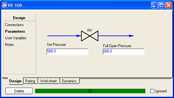
The set pressure is the inlet pressure at which the valve starts to open. If the pressure reaches or exceeds the full open pressure, then the valve will be fully open, allowing material to vent.
Sizing

The following valve control types are available:
- Quick opening: Large increase in flow with a small change in valve stroke.
- Linear: Valve travel is directly proportional to the valve stoke.
- Equal Percentage: Equal increments of valve travel produce an equal percentage in flow change.
The flow rate is also determined by the flow area, and the various discharge coefficients, and are approximately as follows:
LK1, VK1 and KCVK1 are typically equal to the valve opening multiplied by applicable discharge coefficients.
The flow is choked if the pressure ratio exceeds the choking constant which is (2/(CpCv+1)) ^ CpCv/(CpCv-1).
Specifications
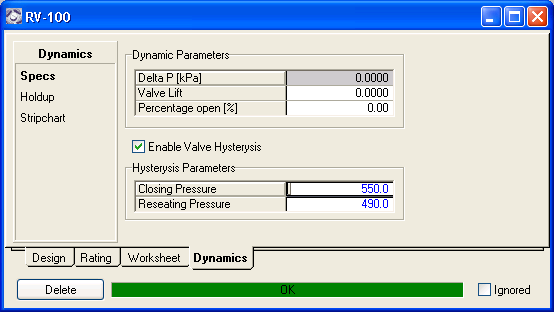
Choose whether the valve opening is directly determined by the pressure only (i.e. the opening will always be the same at a given pressure regardless of whether the valve is opening or closing), or whether it exhibits a more complex hysterysis. In the latter case, the valve opening is also determined by whether the valve is busy opening or closing, and not just by the pressure. This option is commonly used. If the pressure starts to decrease with the valve open, it will start to close at the closing pressure and be fully closed by the time the pressure has dropped to the reseating pressure.
Table of Contents
Introduction
The component splitter is used to model special separation unit operations where the details of how the split is accomplished are not relevant.
Model
In dynamics mode, either fixed split fractions or TBP cut points need to be provided. The Distop model can not be used in dynamics.
The compositonal split is determined by either specifying the component splits directly:

Or by providing them indirectly via TBP splits:

Given that the flows and pressures are determined by the pressure flow network, and the composition by the splits, the stream temperatures still need to be determined:

Checking Calculate Equal Temperatures will iterative solve for the outlet temperature such that the overall heat balance is closed. Checking Use Stream Flash Specifications will allow temperature or other flash specifications to be set in the products. Exactly which specifications become available are also determined by the presence or absence of a duty stream and whether its heatflow value is specified or not. The component splitter will generally close the heat balance.
Specifications

Similar to a mixer or a tee, it is recommended that the Equalize Stream Pressures option be checked. This will link the pressures of all attachment together. If this is not done, there will be no link between the stream pressures, in which case they likely need to be specified in all the streams. This view also shows the various stream pressures as well whether the pressure of a given steam is set to be a specification or not.
A volume can be provided to model a first order compositional response.
Because of the way it works, the component splitter can not handle reverse flow meaningfully. In the case of some flow rates reversing, the component splitter will try to do the most reasonable thing, and may temporarily stop updating streams.
The recycle unit operation is required in steady state to model tear or recycle streams. While it can be used in dynamics mode (where it merely propagates stream information), it is totally redundant and should be removed from flow sheets. It is supported to facilitate easier transition from steady state models.
Dynamics mode handles tear streams automatically, using its own internal mechanisms.
Table of Contents
Introduction
Spreadsheets are fully supported in dynamics mode, and can be used to perform custom calculations or export setpoints to various other operations.
Spreadsheet Dynamics
Spreadsheets continually recalculate (update), as appropriate, in dynamics mode. Their behavior can be set on the dynamics tab in the spreadsheet view:

The first three options determine when and how often the spreadsheet updates (calculates):
- Calculate on Pre Process Step - Calculate before each integration step, frequently.
- Calculate on Post Process Step - Calculate after each integration step, frequently.
- Calculate on Composition Step - Calculate on each composition step, which is typically about ten times less frequently.
Always push outputs determines whether the spreadsheet always pushes all of its exported variables each time it resolves as the integrator runs, or only if one has changed.
Note that spreadsheets do not generate inconsistencies in dynamics mode. The output is generally specified (overridden) so that the user can also change it if need be. If the spreadsheets export an inappropriate value, such as the pressure of a stream that is not set to use a pressure specification, then the spreadsheet exported value will simply be overwritten.
To find out if a spreadsheet is operating on a unit operation, open its view. Then on a blank spot in the view, right click and choose Show Attachments. This will show a list of spreadsheet that are linked to the unit operation in question. Double click on an item in the list to open its view.
For more general information about the spreadsheet, press F1 in Petro-SIM.
Table of Contents
Introduction
This unit operation, which is very similar to a spreadsheet, models a Cause and Effect matrix used in designing and operating plant safety systems. It processes a number of causes and a matrix, and determines the resulting effects.
As a simple example, it can be used to open a valve if a vessel level or vessel pressure exceeds a certain value.
Connections Page

Add causes and effects on this page. Click "Add Causes" or "Add Effects" to use the variable navigator to select a number of variables to be added. Click "Switch" to add a cause which is controlled manually, i.e. not linked to a variable. Similarly, click "Add Effect" to add an effect which is connected to an output object. You can also delete causes and effects from this view, and use the arrow buttons to change the order in which a cause or effect appears in the matrix (and are processed).
You can also add variables to a cause and matrix by right mouse clicking on the variable and choosing to send it to the cause and effect matrix. Or hold the right mouse button down over the "DRAG" text in the cause and effect view, and drop it on a spreadsheet cell or digital switch state for example.
Note that effects generally send 0 or 1 signals. Hence it is common to have a spreadsheet cell or digital unit operation as the output. The valve unit operation also has an on off state variable which translates into a 0% or 100% desired valve opening.
Parameters Page

Global Settings
- Always Update Outputs - Always push an effect output to its associated object, even if the output value has not changed.
- Use Local Switched for Outputs - Lets you manually set the output for all effect.
- Use Output Reset - Any new effects added will have the "Reset?" option checked, and this option will also be checked for all existing effects.
- Bypass All Outputs - Do not send any outputs to the output objects. This can be used during start up or to temporarily disable the matrix.
- Trace All Alarms - Trace alarms in the trace window when they trigger.
- Reset All Outputs - Any outputs with "Reset?" which have tripped, will be reset. Otherwise such effects will remain tripped.
- Hand Pulse Switch Duration - If a cause has a manual switch, you can pulse it on or off for this duration of time.
Cause Variables
- Description - Enter your own user description here.
- Tag - Enter your own tag here.
- Switch - Indicates that this cause is set by a manual switch, its value is not determined by comparing the variable value to the trip value.
- Override - This cause is effectively ignored in calculations.
- Invert - During matrix calculations, the on or off state of this cause is reversed.
- Off Delay - If the variable exceeds the trip, its value must consistently remain above the trip values for this length of time, before it will be treated as having tripped.
- Value - If the cause has a variable, this shows its current value.
- Alarm - If a value is entered, it can be used to raise an alarm if the Value exceeds the Alarm.
- Trip - If a value is entered, the cause will trip if its Value exceeds the Trip value.
- High - If checked, the Value has to the higher than the Alarm and Trip values to trigger, otherwise, lower.
- Pulsed behavior - If the switch option is checked, this can be set. Latched mode means that the switch is manually set and remains at the set value. Pulse On and Pulse Off can be select to have the switch go on or off for a certain length of time only.
- State - Shows the current cause state (Healthy(1) or Tripped(0)).
Effect Variables
- Description - Enter your own user description here.
- Tag - Enter your own tag here.
- Switch - Indicates that this effect is set by a manual switch, and not determined by the matrix outcome.
- Bypass - This cause is effectively ignored in calculations.
- Invert - The reverse of the effect state is sent to the output object.
- Reset? - Indicates that this effect must be reset after it trips, before it can change again.
- Reset - Click here to reset a tripped effect.
- First Out - Shows which cause first tripped this effect.
- Local Switch - Shows the value of the local manual switch, if enabled via the Switch settings.
Matrix Page

The matrix determines which and how certain causes impact an effect. Press the "Legend" button to see the strings. In the screen shot, you can see that for Cause-1 the Value exceeds the Trip value, and hence the input has tripped. The X in the matrix for Cause-1 and Effect-1, indicates that this input will trip Effect-1, as shown. Cause-2 has a green mark in the matrix next to it, indicating that it is healthy. The T5 for it under Effect-1 means that the value of Cause-2 (Vessel Pressure) has to exceed to bound for at least 5 second continuously before it will trip Effect-1.
Table of Contents
Introduction
This section covers the PID, Ratio, Split Range and MPC controllers.
The proportional integral derivative controller (PID controller) is a generic controller widely used in models and in industrial control.
Ratio control is used to ensure that two or more process variables are kept at the same ratio even if they are changing in value. Examples of ratio control include burner air/fuel ratio, blending two liquids, or adjusting heat input in proportion to material flow. For ratio control, a remote setpoint is selected.
Split range control splits an output signal to two or output objects. It is commonly used to control two valves. In a typical configuration, one is fully open while the other is fully closed. If one is 25% open, the other may be 75% open.
Model predictive control (MPC) is an advanced control option which uses a model to predict the behavior of the plant and to accordingly adjust numerous output signals.
Connections

The connections page allows process variable sources and output target objects to be selected. Valve unit operations make ideal output targets because they provide the most realistic and natural response. For a valve output object, the actuator desired position will be controlled, rather than the valve opening (which is a function of various other considerations). For a valve, you can also choose whether to control the main valve, the bypass valve, or either of the two block valves around the main valve.
If the output object is a duty stream or material stream, then click on Control Valve and be sure to supply the minimum and maximum available. These values are used to convert the control signal to a duty or flow rate or other type of value.

Note that some controllers support multiple connections. For example, the split range range controller allows two outputs to be selected. You can change which connection is being shown by using the spinner control  . The ratio controller allows two process variable inputs to be connected.
Parameters - Configuration

The controller Mode determines the behavior of the controller. The following modes may be available, depending on the configuration and type of controller:
- Off - The controller does not perform any calculates and is inactive.
- Man - In manual mode the controller OP is specified directly by the user, and not calculated by the a control algorithm.
- Auto - In automatic mode the controllers operates by itself, adjusting the output based on the various settings.
- Indicator - The controller does not calculate an output value and may not even have an output connection. This mode is also handy for accessing all values via OLE or for just monitoring a value.
- Ramping - This mode is active while the setpoint is temporarily being ramped, as configured and enabled on the Parameters, Advanced page.
- Casc - Cascade control is available when a remote setpoint source has been selected on the connections page. Effectively the output of the primary controller manipulates the setpoint of the secondary controller.
- AutoTune - The controller is currently busy tuning itself. This mode is active when one of the options on the auto tuning page is selected.
The execution can be internal or external. Internal means the Petro-SIM controller code is active. External means that an external DCS or other system is performing control calculations and controller output values are being passed to Petro-SIM via OLE functions or other means.
SP is the target setpoint for the process variable PV. OP shows the current controller output signal.
Kc, Ti and Td and controller algorithm constants that determine the gain, integral and derivative control algorithm contributions.
When applicable, the PV range must be specified. This is used to convert PV values such as temperature into a control signal.
A ratio controller also has an option on this page to enable ratio control. When active, the desired PV ratio can be specified instead of an absolute setpoint.
Ratio Control

The controller should be configured such that PV 1 (as opposed to PV 2) is impacted by the output object of the split range controller (e.g. PV 1 can be flow rate into the valve that is the output object). PV 2 is typically coming from another line or controlled by a different controller. The value of PV 2 is shown as Ref. PV on the Parameters, Operation page. If the Ratio is specified to be 1.5, then PV 2 = Ref.PV = may be equal to 200 say, whereas PV 2, being controlled by the ratio controller, will then be driven to 300. The ratio controller functions just like a regular PID controller, except that its setpoint is calculated as Ratio * Ref.PV, or Ratio * PV 2.
Split Range Control

The split range controller works essentially just like a regular PID controller, except that two output connections are allowed. The setpoint provided is generally that of OP 1 as opposed to OP 2.
Parameters - Configuration

This page is generally used for controllers with multiple connections to allow ranges for the PV and OP values to be provided.
Parameters - Advanced

Set point ramping allows the setpoint to be temporarily boosted or reduced.
SetPoint Options control settings such as whether the SP should update and track the PV value while the controller is in manual mode, or whether to retain its original value.
The limit values are used inside the control algorithms to convert values values to signals.
Four algorithms are available:
- PID Velocity Form
- PID Positional Form (ARW)
- PID Positional Form (NoARW)
- PID Manual Loading
The velocity form is incremental, dealing with rate of change. The positional form deals with values which are actual position (e.g. valve opening) value.
ARW refers to the presence of anti-reset windup, which can be a problem if the control loop is temporarily taken out of control. During such times the integral portion of the control can rise to high values (wind up), which lengthens the time it takes the control loop to get back to minimal error. The term "wind-up" is a way of viewing the integral term as a spring that takes a long time to "unwind".
Auto Tune

While the integrator is running (and the process is fairly lined out with the controller PV close to the setpoint) click on Start Autotuner. This will perform some response testing and calculate tuning parameters for the controller. Click Accept to accept the new parameters.
The auto tuner will automatically exit auto tuning mode once it has calculated new parameters, a process that generally does not take long. But if the process conditions are not suitable, the controller can be taken out of auto tuning mode by clicking Stop Autotuning.
Note that is unlikely that any automatic tuning will by default produce the exact desired response. But properly used, auto tuning can be very helpful.
The autotuner calculates the amplitude and period of oscillation. For a PI controller the values are calculated as follows:
For a PID controller the equations are as follows:
IMC Design

This is an internal model control (IMC) based single-loop controller design method. Effectively, another way of tuning the controller. If values for the process gain, process time constant, process delay, and design Tc (the closed loop time constant) are known, entering them will calculate PID tuning parameters. These values can be determined by doing step testing, as described by numerous authors.
Scheduling

Based on either the PV or SP, it is possible to have three sets of controller tuning parameters and have the controller automatically flip between them.
Alarms

It is possible to define low low, low, high and high high alarms, for the controller PV (process variable), OP (output), SP (setpoint), DV (disturbance variable) and the RS (remote setpoint) signals. These alarms are displayed by the controller in its view as well as in the left bottom status view of Petro-SIM.
The deadband is used to prevent an alarm from going on and off repeatedly if the value varies close to the alarm value.
PV Conditioning

Control signals can fail in numerous ways or be off for some reason or another. The controller can also simulate these failures:
- None - The true PV value is used by the controller.
- Fixed Signal - The PV value fails to a specific value or freezes at the value it has at the time of failure.
- Bias - The PV signal has a fixed offset, or is drifting over time.
In addition, the PV can be sampled only so often and held fixed when not sampled.
Signal Processing

A filter and noise can be applied to a controller signal. The filter effectively repeatedly averages the signal with the filter value over time, depending on the filter time. The noise is randomly added and as such may result in a simulation not being completely reproducible if restarted.
Note that while these may be useful in providing modeling realism, they are not frequently used.
Feed Forward
Feed forward control measures disturbances to improve control. The gain (Kp), time delay, and time constants of the process must be specified.
MPC
Model predictive control, which generally controls all the outputs of a plant section or unit operation, allows for very efficient control, if it has a good model of the process.
The MPC controller in Petro-SIM, which allows experimentation with MPC control, will be supported in future releases.
Table of Contents

Introduction
In additional to the spreadsheet, cause and effect matrix and event scheduler, Petro-SIM also provides an additional range of operations for implemented process logic.
Set

The set operation maintains a relationship between two variables. For example, one stream pressure can be set to be always 10 kPa higher than another. In steady state it calculates either the source target or offset, depending on what is known. In dynamics mode, since all variables are always known, the multiplier and offset are always specified, and the target value is always updated from the source, if need be. Generally the target is a specified variable, whose value is then updated.
Selector

The selector accept a number of input variable sources and based on its settings, determines one output value.


It can calculate the minimum, maximum, median, average, sum, product or quotient (first value divided by all the others). A hand selection (Hand Sel) option is available for selecting a specific input. For each input value as well as the output value, a gain and bias can be applied (PV used = Gain * PV + Bias).
Transfer Function
The transfer function operation (signal block) can be used to implement or effect control transfer functions, and allows a combination of integrator, lead, lag and second order functions to be combined. The integrator option sums up: InputSignal * StepSize / Integrator Period.
Digital Point

The digital point takes an optional variable source and an optional output target. It can be Off, in Manual mode, or in Automatic mode.
Manual mode: If the operation is latched, the output will be On or Off as set and remain so. If the operation is set to pulsed mode, it can temporarily pulse on or off. For example, if the Output is set to On, and the operation is set to Pulse Off with a pulse duration of 2 seconds, then clicking on Off will send an Off (zero) output signal for two seconds before the digital point will revert back to being On.
Automatic mode: The PV value is compared with a threshold and the digital point is either on or off or pulsed for the duration depending on the result of the comparison.
The digital point can also show alarms based on the PV value. The deadband is used to ensure that an alarm does not rapidly cycle between on and off if the PV value is closed to the alarm value.
The digital point is also an easy way to for example turn pumps in the flowsheet on or off.
Boolean Not Gate

The Not gate takes a single input, reverses its value, and sends it to one or more outputs.
Boolean And Gate

The And gate send a true output only if all inputs are true. If any one is false, its output is false as well.
Boolean Or Gate
The Or gate send a true output if one or more of the inputs are true. If they are all false, its output is false as well.
Boolean XOr gate
The XOr gate send a false output if all inputs are either false, or all inputs are true. If some but not all inputs are true, ts output is true as well.
Boolean OffDly Gate

This unit operatoin waits the designated amount of time before passing an on value through.
Boolean OnDly Gate
This unit operatoin waits the designated amount of time before passing an off value through.
Boolean Latch Gate

If there is only one process variable source, then it determines the latch value.
If there are two process variable sources, then the first one sets the latch (makes its output go to true and stay there) and the second one resets it (makes the output go back to false again) it. Assume both inputs are false, and the latch is zero (output is zero). If the first input goes to true, the latch output will go to true and remain there even if the first input goes to false again. It will reset (go to false) only if the second input goes to true (provided the first input is not true anymore either).
Boolean CountUp Gate
Two inputs are required. The second input acts as a reset flag, and if true, it reverses the output value. If it is false, the first input value is compared with the output alarm. If it is equal then the current counter is incremented. If the Current Counter reaches the Maximum Counter, then the Output value gets pushed out.
Boolean CountDown Gate
This works similar to the count up gate, except that when the fitst input is compared with the output alarm and is equal, then the current counter gets decremented instead of incremented.
Adjust
The adjust unit operation adjusts one variable to drive another towards a specific target. In dynamics mode, doing this is far more complicated because timing and transient phenomena play a role as well. Hence adjust unit operations are ineffective in dynamics mode. Use a controller instead.
Table of Contents
Introduction
This section contains advanced or requested special topics. These topics currently are:
Feedback
This documentation was written with the aim of providing useful content, and not just to have documentation or copy what is in the views already. KBC appreciates your feedback. If you have found this documentation useful, or if you have improvements or suggestions for the documentation, or was looking for a specific topic on this page, please do let us know. You can send an email to: software at kbcat.com. Ask for it to be forwarded to Ben.
Table of Contents
Introduction
Dynamics mode supports three phases, and stores each in a different slot, and keeps track of each phase. It can happen that part of the simulation has only one liquid phase and other parts of it have two liquid phases. The flash by default also uses arbitrary cut-off rules to determine whether a phase is aqueous or not, and that can cause the order of phases returned by the flash to suddenly change. This can cause severe model instability and you can best see this on the vessel phases page:
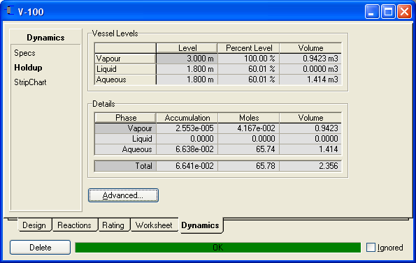
If the liquid levels and moles flip between the second and third slots as the integrator runs, then the case has a phase sorting problem.
Configuration
This problem can best be dealt with by using the phase sorting options of the fluid package in the basis environment:

These settings allow a custom definition of when a liquid phase should be in slot1 versus slot 2. It should be set up in such a way that the same phase will always end up in the same slot throughout the model (i.e. no phase flipping).
It is generally recommended that the phase sorting option be applied to avoid the possibility of this type of problem.
When controlling a composition or temperature, it is common to choose the PV from a stream. However, this can be problematic if the flow is very low, stopped, or reversed. In such situations the variable will stop responding to the manipulated variable, but the controller may continue to boost its output signal. So be careful what stream is chosen, or try and obtain the variable from a vessel.
This documentation was written with the aim of providing useful content, and not just to have documentation or copy what is in the views already. KBC appreciates your feedback. If you have found this documentation useful, or if you have improvements or suggestions for the documentation, or was looking for a specific topic on this page, please do let us know. You can send an email to software@kbcat.com. Ask for it to be forwarded to Ben.